
DistilBart is a typical encoder-decoder model for NLP tasks. In this tutorial, you will learn how such a model is constructed and how you can check its architecture so that you can compare it with other models. You will also learn how to use the pretrained DistilBart model to generate summaries and how to control the summaries’ style.
After completing this tutorial, you will know:
- How DistilBart’s encoder-decoder architecture processes text internally
- Methods for controlling summary style and content
- Techniques for evaluating and improving summary quality
Let’s get started!
Understanding the DistilBart Model and ROUGE Metric
Photo by Svetlana Gumerova. Some rights reserved.
Overview
This post is in two parts; they are:
- Understanding the Encoder-Decoder Architecture
- Evaluating the Result of Summarization using ROUGE
Understanding the Encoder-Decoder Architecture
DistilBart is a “distilled” version of the BART model, a powerful sequence-to-sequence model for natural language generation, translation, and comprehension. The BART model uses a full transformer architecture with an encoder and decoder.
You can find the architecture of transformer models in the paper Attention is all you need. At a high level, the illustration is as follows:
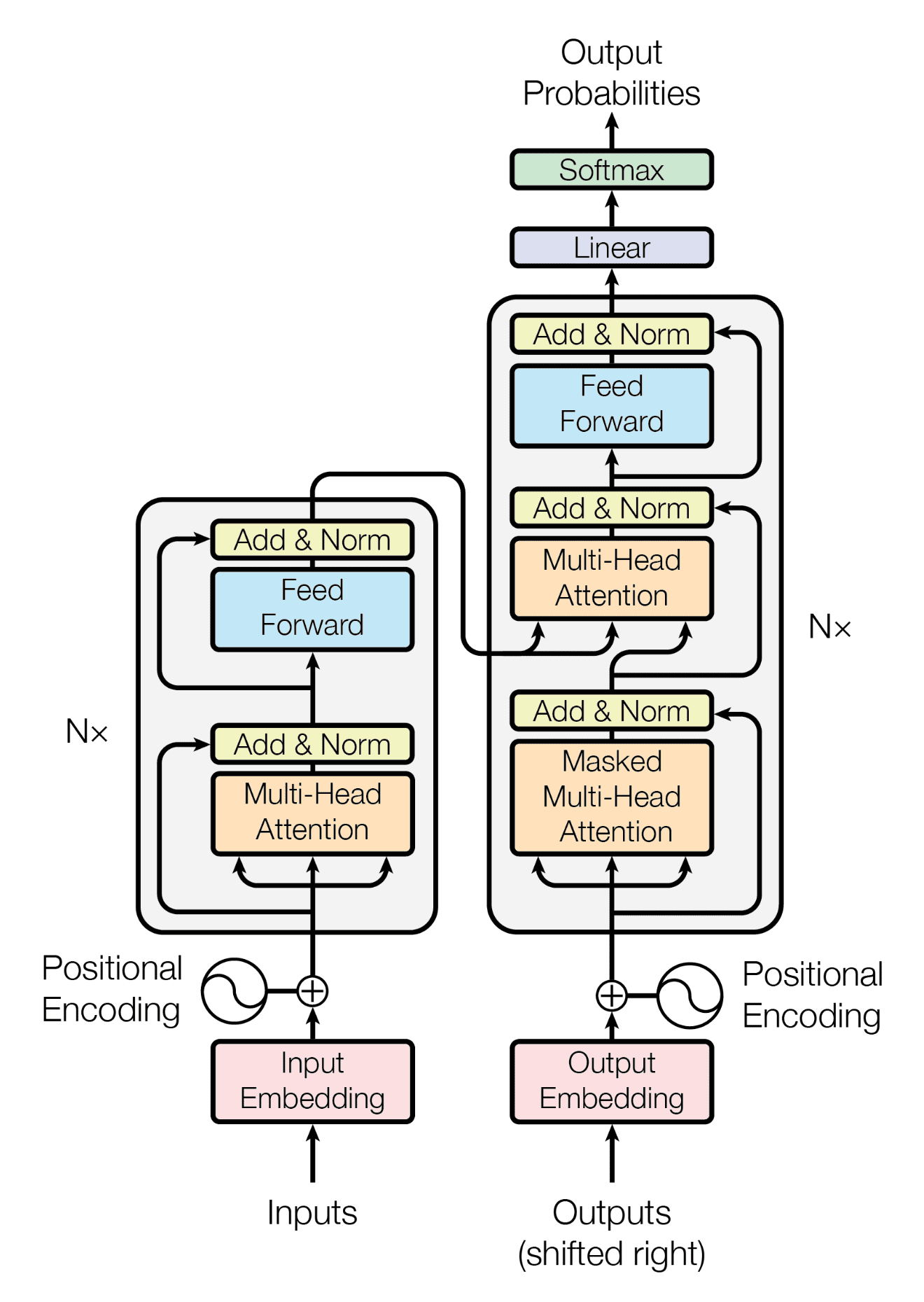
Transformer architecture
The key characteristic of the transformer architecture is that it is split into an encoder and a decoder. The encoder takes the input sequence and outputs a sequence of hidden states. The decoder takes the hidden states and outputs the final sequence. It is very effective for sequence-to-sequence tasks like summarization, in which the input should be fully consumed to extract the key information before the summary can be generated.
As explained in the previous post, you can use the pretrained DistilBart model to build a summarizer with just a few lines of code. In fact, you can see some of the design parameters in DistilBart’s architecture by looking at the model config:
|
1 2 3 4 5 6 7 8 9 10 11 12 13 14 15 16 17 18 19 20 21 22 23 |
rom transformers import AutoConfig, AutoModelForSeq2SeqLM
def explore_model_architecture(): “”“Examine DistilBart’s configuration and architecture.”“” model_name = “sshleifer/distilbart-cnn-12-6”
# Load model configuration config = AutoConfig.from_pretrained(model_name) print(“Model Architecture:”) print(f“- Encoder layers: {config.encoder_layers}”) print(f“- Decoder layers: {config.decoder_layers}”) print(f“- Hidden size: {config.hidden_size}”) print(f“- Attention heads: {config.encoder_attention_heads}”)
# Verify encoder-decoder structure model = AutoModelForSeq2SeqLM.from_pretrained(model_name) print(“\nModel Components:”) print(f“- Encoder: {type(model.model.encoder).__name__}”) print(f“- Decoder: {type(model.model.decoder).__name__}”) return model, config
# Example usage model, config = explore_model_architecture() |
The code above prints the size of the hidden state, the number of attention heads, and the number of encoder and decoder layers i
|
Model Architecture: – Encoder layers: 12 – Decoder layers: 6 – Hidden size: 1024 – Attention heads: 16 Model Components: – Encoder: BartEncoder – Decoder: BartDecoder |
The model created in this way is a PyTorch model. You can print the model if you want to see more:
Which should show you:
|
1 2 3 4 5 6 7 8 9 10 11 12 13 14 15 16 17 18 19 20 21 22 23 24 25 26 27 28 29 30 31 32 33 34 35 36 37 38 39 40 41 42 43 44 45 46 47 48 49 50 51 52 53 |
artForConditionalGeneration( (model): BartModel( (shared): BartScaledWordEmbedding(50264, 1024, padding_idx=1) (encoder): BartEncoder( (embed_tokens): BartScaledWordEmbedding(50264, 1024, padding_idx=1) (embed_positions): BartLearnedPositionalEmbedding(1026, 1024) (layers): ModuleList( (0-11): 12 x BartEncoderLayer( (self_attn): BartSdpaAttention( (k_proj): Linear(in_features=1024, out_features=1024, bias=True) (v_proj): Linear(in_features=1024, out_features=1024, bias=True) (q_proj): Linear(in_features=1024, out_features=1024, bias=True) (out_proj): Linear(in_features=1024, out_features=1024, bias=True) ) (self_attn_layer_norm): LayerNorm((1024,), eps=1e-05, elementwise_affine=True) (activation_fn): GELUActivation() (fc1): Linear(in_features=1024, out_features=4096, bias=True) (fc2): Linear(in_features=4096, out_features=1024, bias=True) (final_layer_norm): LayerNorm((1024,), eps=1e-05, elementwise_affine=True) ) ) (layernorm_embedding): LayerNorm((1024,), eps=1e-05, elementwise_affine=True) ) (decoder): BartDecoder( (embed_tokens): BartScaledWordEmbedding(50264, 1024, padding_idx=1) (embed_positions): BartLearnedPositionalEmbedding(1026, 1024) (layers): ModuleList( (0-5): 6 x BartDecoderLayer( (self_attn): BartSdpaAttention( (k_proj): Linear(in_features=1024, out_features=1024, bias=True) (v_proj): Linear(in_features=1024, out_features=1024, bias=True) (q_proj): Linear(in_features=1024, out_features=1024, bias=True) (out_proj): Linear(in_features=1024, out_features=1024, bias=True) ) (activation_fn): GELUActivation() (self_attn_layer_norm): LayerNorm((1024,), eps=1e-05, elementwise_affine=True) (encoder_attn): BartSdpaAttention( (k_proj): Linear(in_features=1024, out_features=1024, bias=True) (v_proj): Linear(in_features=1024, out_features=1024, bias=True) (q_proj): Linear(in_features=1024, out_features=1024, bias=True) (out_proj): Linear(in_features=1024, out_features=1024, bias=True) ) (encoder_attn_layer_norm): LayerNorm((1024,), eps=1e-05, elementwise_affine=True) (fc1): Linear(in_features=1024, out_features=4096, bias=True) (fc2): Linear(in_features=4096, out_features=1024, bias=True) (final_layer_norm): LayerNorm((1024,), eps=1e-05, elementwise_affine=True) ) ) (layernorm_embedding): LayerNorm((1024,), eps=1e-05, elementwise_affine=True) ) ) (lm_head): Linear(in_features=1024, out_features=50264, bias=False) ) |
This may not be easy to read. But if you are familiar with the transformer architecture, you will notice that:
- The
BartModelhas an embedding model, an encoder model, and a decoder model. The same embedding model appears in both the encoder and decoder. - The size of the embedding model suggests that the vocabulary contains 50264 tokens. The output of the embedding model has a size of 1024 (the “hidden size”), which is the length of the embedding vector for each token.
- Both the encoder and decoder use the
BartLearnedPositionalEmbeddingmodel, which presumably is a learned positional encoding for the input sequence to each model. - The encoder has 12 layers and the decoder has only 6 layers. Note that DistilBart is a “distilled” version of BART because BART has 12 layers of decoder but DistilBart simplified it into 6.
- In each layer of the encoder, there is one self-attention, two layer norms, two feed-forward layers, and using GELU as the activation function.
- In each layer of the decoder, there is one self-attention, one cross-attention from the encoder, three layer norms, two feed-forward layers, and using GELU as the activation function.
- In both the encoder and decoder, the hidden size does not change through the layers, but the feed-forward layer uses 4x the hidden size in the middle.
Most transformer models use a similar architecture but with some variations. These are the high-level building blocks of the model, but you cannot see the exact algorithm used, for example, the order of the building blocks invoked with the input sequence. You can find such details only when you check the model implementation code.
Not all models have both an encoder and a decoder. However, this design is very common for sequence-to-sequence tasks. The output from the encoder model is called the “contextual representation” of the input sequence. It captures the essence of the input text. The decoder model uses the contextual representation to generate the final sequence.
Evaluating the Result of Summarization using ROUGE
As you have seen how to use the pretrained DistilBart model to generate summaries, how do you know the quality of its output?
This is indeed a very difficult question. Everyone has their own opinion on what a good summary is. However, some well-known metrics are used to evaluate various outputs of language models. One popular metric for evaluating the quality of summaries is ROUGE.
ROUGE stands for Recall-Oriented Understudy for Gisting Evaluation. It is a set of metrics used to evaluate the quality of text summarization and machine translation. Behind the scenes, the F1 score of the precision and recall of the generated summary is computed against the reference summary. It is simple to understand and easy to compute. As a recall-based metric, it focuses on the ability of the summary to recall the key phases. The weakness of ROUGE is that it needs a reference summary. Hence, the effectiveness of the evaluation depends on the quality of the reference.
Let’s revisit how we can use DistilBart to generate summaries:
|
1 2 3 4 5 6 7 8 9 10 11 12 13 14 15 16 17 18 19 20 21 22 23 24 25 26 27 28 29 30 31 32 33 34 35 36 37 38 39 40 41 42 43 44 45 46 47 48 |
import torch from transformers import AutoTokenizer, AutoModelForSeq2SeqLM
class Summarizer: def __init__(self, model_name=“sshleifer/distilbart-cnn-12-6”): “”“Initialize the summarizer with model and tokenizer.”“” self.device = “cuda” if torch.cuda.is_available() else “cpu” self.tokenizer = AutoTokenizer.from_pretrained(model_name) self.model = AutoModelForSeq2SeqLM.from_pretrained(model_name) self.model.to(self.device)
def summarize(self, text, context_weight=0.5, max_length=150, min_length=50, num_beams=4, length_penalty=2.0, repetition_penalty=1.0, do_sample=False, temperature=1.0, early_stopping=True): “”“Generate a summary with context awareness.”“” inputs = self.tokenizer(text, return_tensors=“pt”, padding=True, truncation=True, max_length=1024 ).to(self.device) # Generate summary using only the input tokens summary_ids = self.model.generate( inputs[“input_ids”], attention_mask=inputs[“attention_mask”], max_length=max_length, min_length=min_length, num_beams=num_beams, length_penalty=length_penalty, repetition_penalty=repetition_penalty, do_sample=do_sample, temperature=temperature, early_stopping=early_stopping, ) # Decode and return the summary summary = self.tokenizer.decode(summary_ids[0], skip_special_tokens=True) return summary
# Let’s run an example to see how it works summarizer = Summarizer() text = “”“ The development of artificial intelligence has revolutionized numerous industries. Machine learning algorithms now power everything from recommendation systems to autonomous vehicles. Deep learning, in particular, has shown remarkable success in tasks like image recognition and natural language processing. However, these advances also raise important ethical considerations about AI’s impact on society, privacy, and employment. ““”
summary = summarizer.summarize(text) print(f“Summary:\n{summary}”) |
The Summarizer class loads the pretrained DistilBart model and tokenizer and then uses the model to generate a summary of the input text. To generate the summary, several parameters are passed to the generate() method to control how the summary is generated. You can adjust these parameters, but the default values are a good starting point.
Now let’s extend the Summarizer class to generate summaries with different styles by setting different parameters for the generate() method:
|
1 2 3 4 5 6 7 8 9 10 11 12 13 14 15 16 17 18 19 20 21 22 23 24 25 26 27 28 29 30 31 32 33 34 35 36 37 38 39 40 41 42 43 44 45 46 47 48 49 50 51 52 53 54 55 56 57 58 59 60 61 62 63 |
..
class StyleControlledSummarizer(Summarizer): def summarize_with_style(self, text, style=“concise”): “”“Generate summaries with different styles.
Args: text (str): Input text to summarize style (str): Summary style (‘concise’, ‘detailed’, ‘technical’, ‘simple’) Returns: str: Generated summary with specified style ““” style_params = { “concise”: { “max_length”: 80, “min_length”: 30, “length_penalty”: 3.0, “num_beams”: 4, “early_stopping”: True }, “detailed”: { “max_length”: 200, “min_length”: 100, “length_penalty”: 1.0, “num_beams”: 6, “early_stopping”: False }, “technical”: { “max_length”: 150, “min_length”: 50, “length_penalty”: 2.0, “num_beams”: 5, “repetition_penalty”: 1.5 }, “simple”: { “max_length”: 100, “min_length”: 30, “length_penalty”: 2.0, “num_beams”: 3, “do_sample”: True, “temperature”: 0.7 } } params = style_params[style] return self.summarize(text, **params)
# Let’s run an example to see how it works style_summarizer = StyleControlledSummarizer() text = “”“ Quantum computing leverages the principles of quantum mechanics to perform computations. Unlike classical computers that use bits, quantum computers use quantum bits or qubits. These qubits can exist in multiple states simultaneously through superposition, potentially allowing quantum computers to solve certain problems exponentially faster than classical computers. However, maintaining quantum coherence and minimizing errors remains a significant challenge in building practical quantum computers. ““”
styles = [“concise”, “detailed”, “technical”, “simple”] for style in styles: summary = style_summarizer.summarize_with_style(text, style=style) print(f“\n{style.capitalize()} Summary:”) print(summary) |
The StyleControlledSummarizer class defined four styles of summaries, named “concise”, “detailed”, “technical”, and “simple”. You can see that the parameters for the generate() method differ for each style. In particular, the “detailed” style uses a longer summary length, the “technical” style uses a higher repetition penalty, and the “simple” style uses a lower temperature for more creative summaries.
Is that good? Let’s see what the ROUGE metric says:
|
1 2 3 4 5 6 7 8 9 10 11 12 13 14 15 16 17 18 19 20 21 22 23 24 25 26 27 28 29 30 31 32 33 34 35 36 37 38 |
...
from rouge_score import rouge_scorer
class SummaryEvaluator: def __init__(self): “”“Initialize with ROUGE metrics.”“” self.scorer = rouge_scorer.RougeScorer( [‘rouge1’, ‘rouge2’, ‘rougeL’], use_stemmer=True )
def evaluate_summary(self, reference, candidate): “”“Calculate ROUGE scores for a summary.
Args: reference (str): Reference summary candidate (str): Generated summary
Returns: dict: ROUGE scores for different metrics ““” scores = self.scorer.score(reference, candidate)
print(“Summary Quality Metrics:”) print(f“ROUGE-1: {scores[‘rouge1’].fmeasure:.3f}”) print(f“ROUGE-2: {scores[‘rouge2’].fmeasure:.3f}”) print(f“ROUGE-L: {scores[‘rougeL’].fmeasure:.3f}”)
return scores
# Checking the matrics implementation summarizer = StyleControlledSummarizer() evaluator = SummaryEvaluator() reference = “Quantum computing uses qubits for faster computation but faces coherence challenges.” for style in [“concise”, “detailed”, “technical”, “simple”]: candidate = summarizer.summarize_with_style(text, style=style) scores = evaluator.evaluate_summary(reference, candidate) |
You may see the output like this:
|
1 2 3 4 5 6 7 8 9 10 11 12 13 14 15 16 17 18 19 20 21 22 23 24 25 26 27 28 29 30 31 32 33 34 35 36 37 38 39 40 41 42 43 44 |
Concise Summary: Quantum computing leverages the principles of quantum mechanics to perform certain problems exponentially faster than classical computers . Unlike classical computers that use bits, quantum computers use quantum bits or qubits . These qubits can exist in multiple states simultaneously through superposition . Summary Quality Metrics: ROUGE-1: 0.235 ROUGE-2: 0.082 ROUGE-L: 0.157
Detailed Summary: Quantum computing leverages the principles of quantum mechanics to perform quantum computations . Unlike classical computers that use bits, quantum computers use quantum bits or qubits . These qubits can exist in multiple states simultaneously through superposition, potentially allowing quantum computers to solve certain problems exponentially faster than classical computers . However, maintaining quantum coherence and minimizing errors remains a significant challenge in building practical quantum computers, according to the University of Cambridge, UK, researchers . Back to Mail Online home .Back to the page you came from . Summary Quality Metrics: ROUGE-1: 0.168 ROUGE-2: 0.043 ROUGE-L: 0.168
Technical Summary: Quantum computing leverages the principles of quantum mechanics to perform certain problems exponentially faster than classical computers . Unlike classical computers that use bits, quantum computers use quantum bits or qubits . These qubits can exist in multiple states simultaneously through superposition . However, maintaining quantum coherence and minimizing errors remains a challenge . Summary Quality Metrics: ROUGE-1: 0.262 ROUGE-2: 0.068 ROUGE-L: 0.197
Simple Summary: Quantum computing leverages the principles of quantum mechanics to perform quantum computing . Unlike classical computers that use bits, quantum computers use quantum bits or qubits . These qubits can exist in multiple states simultaneously through superposition . Summary Quality Metrics: ROUGE-1: 0.217 ROUGE-2: 0.091 ROUGE-L: 0.174 |
To run this code, you need to install the rouge_score package:
Three metrics are used above. ROUGE-1 is based on unigrams, i.e., single words. ROUGE-2 is based on bigrams, i.e., two words. ROUGE-L is based on the longest common subsequence. Each metric measures different aspects of summary quality. The higher the metric, the better.
As you can see from the above, a longer summary is not always better. It all depends on the “reference” you used to evaluate the ROUGE metrics.
Putting it all together, below is the complete code:
|
1 2 3 4 5 6 7 8 9 10 11 12 13 14 15 16 17 18 19 20 21 22 23 24 25 26 27 28 29 30 31 32 33 34 35 36 37 38 39 40 41 42 43 44 45 46 47 48 49 50 51 52 53 54 55 56 57 58 59 60 61 62 63 64 65 66 67 68 69 70 71 72 73 74 75 76 77 78 79 80 81 82 83 84 85 86 87 88 89 90 91 92 93 94 95 96 97 98 99 100 101 102 103 104 105 106 107 108 109 110 111 112 113 114 115 116 117 118 119 120 121 122 123 124 125 |
import torch from rouge_score import rouge_scorer from transformers import AutoTokenizer, AutoModelForSeq2SeqLM
class Summarizer: def __init__(self, model_name=“sshleifer/distilbart-cnn-12-6”): “”“Initialize the summarizer with model and tokenizer.”“” self.device = “cuda” if torch.cuda.is_available() else “cpu” self.tokenizer = AutoTokenizer.from_pretrained(model_name) self.model = AutoModelForSeq2SeqLM.from_pretrained(model_name) self.model.to(self.device)
def summarize(self, text, context_weight=0.5, max_length=150, min_length=50, num_beams=4, length_penalty=2.0, repetition_penalty=1.0, do_sample=False, temperature=1.0, early_stopping=True): “”“Generate a summary with context awareness.”“” inputs = self.tokenizer(text, return_tensors=“pt”, padding=True, truncation=True, max_length=1024 ).to(self.device) # Generate summary using only the input tokens summary_ids = self.model.generate( inputs[“input_ids”], attention_mask=inputs[“attention_mask”], max_length=max_length, min_length=min_length, num_beams=num_beams, length_penalty=length_penalty, repetition_penalty=repetition_penalty, do_sample=do_sample, temperature=temperature, early_stopping=early_stopping, ) # Decode and return the summary summary = self.tokenizer.decode(summary_ids[0], skip_special_tokens=True) return summary
class StyleControlledSummarizer(Summarizer): def summarize_with_style(self, text, style=“concise”): “”“Generate summaries with different styles.
Args: text (str): Input text to summarize style (str): Summary style (‘concise’, ‘detailed’, ‘technical’, ‘simple’) Returns: str: Generated summary with specified style ““” style_params = { “concise”: { “max_length”: 80, “min_length”: 30, “length_penalty”: 3.0, “num_beams”: 4, “early_stopping”: True }, “detailed”: { “max_length”: 200, “min_length”: 100, “length_penalty”: 1.0, “num_beams”: 6, “early_stopping”: False }, “technical”: { “max_length”: 150, “min_length”: 50, “length_penalty”: 2.0, “num_beams”: 5, “repetition_penalty”: 1.5 }, “simple”: { “max_length”: 100, “min_length”: 30, “length_penalty”: 2.0, “num_beams”: 3, “do_sample”: True, “temperature”: 0.7 } } params = style_params[style] return self.summarize(text, **params)
class SummaryEvaluator: def __init__(self): “”“Initialize with ROUGE metrics.”“” self.scorer = rouge_scorer.RougeScorer( [‘rouge1’, ‘rouge2’, ‘rougeL’], use_stemmer=True )
def evaluate_summary(self, reference, candidate): “”“Calculate ROUGE scores for a summary.
Args: reference (str): Reference summary candidate (str): Generated summary
Returns: dict: ROUGE scores for different metrics ““” scores = self.scorer.score(reference, candidate)
print(“Summary Quality Metrics:”) print(f“ROUGE-1: {scores[‘rouge1’].fmeasure:.3f}”) print(f“ROUGE-2: {scores[‘rouge2’].fmeasure:.3f}”) print(f“ROUGE-L: {scores[‘rougeL’].fmeasure:.3f}”)
return scores
# Checking the matrics implementation summarizer = StyleControlledSummarizer() evaluator = SummaryEvaluator() text = “”“ Quantum computing leverages the principles of quantum mechanics to perform computations. Unlike classical computers that use bits, quantum computers use quantum bits or qubits. These qubits can exist in multiple states simultaneously through superposition, potentially allowing quantum computers to solve certain problems exponentially faster than classical computers. However, maintaining quantum coherence and minimizing errors remains a significant challenge in building practical quantum computers. ““” reference = “Quantum computing uses qubits for faster computation but faces coherence challenges.” for style in [“concise”, “detailed”, “technical”, “simple”]: summary = summarizer.summarize_with_style(text, style=style) print(f“\n{style.capitalize()} Summary:”) print(summary) scores = evaluator.evaluate_summary(reference, summary) |
Further Reading
Below are some resources that you may find useful:
- DistilBart Model
- ROUGE Metric
- Pre-trained Summarization Distillation by Sam Shleifer, Alexander M. Rush (arXiv:2010.13002)
- BART: Denoising Sequence-to-Sequence Pre-training for Natural Language Generation, Translation, and Comprehension by Mike Lewis, Yinhan Liu, Naman Goyal, Marjan Ghazvininejad, Abdelrahman Mohamed, Omer Levy, Ves Stoyanov, Luke Zettlemoyer (arXiv:1910.13461)
- Attention is all you need by Ashish Vaswani, Noam Shazeer, Niki Parmar, Jakob Uszkoreit, Llion Jones, Aidan N. Gomez, Lukasz Kaiser, Illia Polosukhin (arXiv:1706.03762)
- Chin-Yew Lin. 2004. ROUGE: A Package for Automatic Evaluation of Summaries. In Text Summarization Branches Out, pages 74–81, Barcelona, Spain. Association for Computational Linguistics.
Summary
In this advanced tutorial, you’ve learned several advanced features of text summarization. Particularly, you learned:
- How DistilBart’s encoder-decoder architecture processes text
- Methods for controlling summary style
- Approaches to evaluating summary quality
These advanced techniques enable you to create more sophisticated and effective text summarization systems tailored to specific needs and requirements.