Image by Author | Canva Pro
Are you seeking a cutting-edge model like GPT-4o for time series forecasting? Enter TimeGPT, a Transformer-based model trained on general time series datasets. You can fine-tune it on your dataset to achieve state-of-the-art performance with few lines of code.
In this tutorial, we will explore TimeGPT and the Nixtla API. We will learn simple and advanced forecasting techniques using the Nixtla Python package. Finally, we will evaluate model performance with the Nixtla ecosystem.
This straightforward guide is perfect for anyone looking to enhance their forecasting skills.
What is TimeGPT?
TimeGPT is a state-of-the-art time series model offering fairly accurate forecasting on unseen datasets. It is a Transformer-based model with a self-attention mechanism that was trained on the largest publicly available time series data collection. This allows TimeGPT to excel in zero-shot inference without retraining, surpassing traditional statistical, machine learning, and deep learning methods in performance, efficiency, and simplicity.
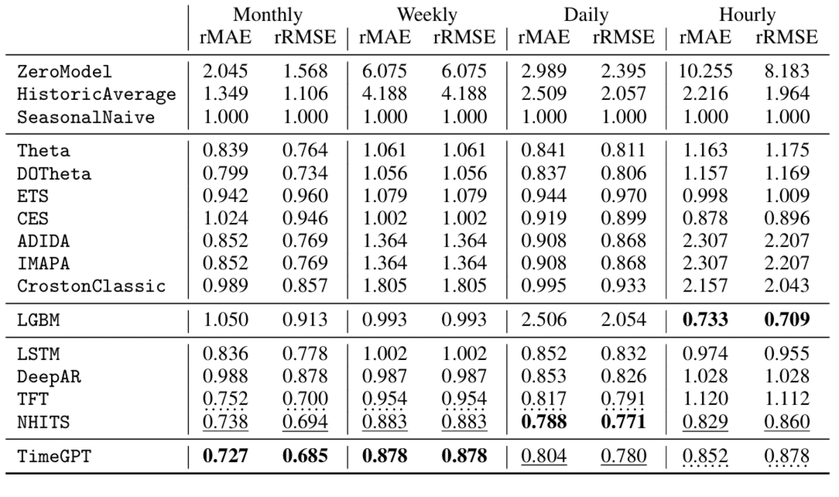

Image from 2310.03589 (arxiv.org)
Getting Started with TimeGPT
To use TimeGPT, we have to generate the Nixtla API by going to the dashboard.nixtla.io website. Click on “Create New API Key” and copy the generated API key.
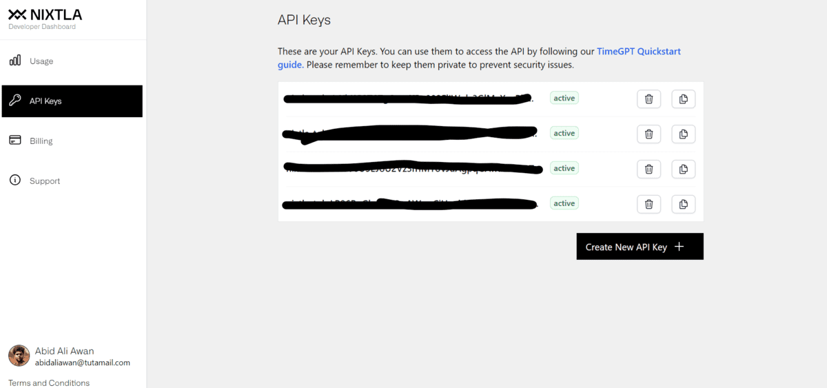

You can set the environment variable with the Nixtla API key. In our case, we are using Deepnote. To set up the environment variable, you have to click on the “+” button on the Integration tab, then select the environment variable option. Provide the Key name and the value, and press the “Create Integration” button.


Install the `yfinance` for stock market data and `nixtla` for the TimeGPT Python client.
%%capture
%pip install nixtla>=0.5.1
%pip install yfinance
Initialize the Nixtla client with the TimeGPT API key.
from nixtla import NixtlaClient
import os

timegpt_api_key = os.environ["TIMEGPT_API_KEY"]

# Setup NixtlaClient
nixtla_client = NixtlaClient(api_key=timegpt_api_key)
Simple Forecasting with TimeGPT
We will download and load the Meta stock market data from the `yfinance` package, and we will only use the last 1000 rows so that we have the latest information for the model to understand.
import pandas as pd
import yfinance as yf

# Downloading Meta stock price data
ticker="META"
meta_stock_data = yf.download(ticker)
meta_stock_data = meta_stock_data.reset_index()
meta_stock_data = meta_stock_data.tail(1000)

# Displaying the dataset
meta_stock_data.head()


Plot the time series data by providing the “Date” and “Adj Close” columns.
nixtla_client.plot(meta_stock_data, time_col="Date", target_col="Adj Close")


To forecast the Meta stock price, we will use the ‘.forecast` function and provide it with the dataset, model name, forecast horizon (h), frequency (only business days), and time and target column.
meta_stock_forecast = nixtla_client.forecast(
    df=meta_stock_data,
    model="timegpt-1",
    h=12,
    freq="B",
    time_col="Date",
    target_col="Adj Close",
)
meta_stock_forecast.tail()
The `.forecast` function will fine-tune the model on our data and return the pandas dataset with the time and forecast column. As we can see, we have successfully forecast the 12 values.


To visualize the results, we will plot both actual and forecast series and only show the last 30 values to give more zoomed-in visualization.
nixtla_client.plot(
    meta_stock_data,
    meta_stock_forecast,
    time_col="Date",
    target_col="Adj Close",
    max_insample_length=30,
)


Advanced Forecasting with TimeGPT
The `.forecast` function also lets you provide more options to fine-tune and improve your results. In the example below, we will generate a 90% confidence interval, fine-tune the model for 120 steps, select a different fine-tuning loss, and add history. This means the forecast will include previous values as well as future values.
meta_stock_forecast = nixtla_client.forecast(
    df=meta_stock_data,
    model="timegpt-1",
    h=12,
    level=[90],  # Generate a 90% confidence interval
    finetune_steps=120,  # Specify the number of steps for fine-tuning
    finetune_loss="mae",  # Specify the loss function for fine-tuning
    freq="B",
    time_col="Date",
    target_col="Adj Close",
    add_history=True
)
meta_stock_forecast.tail()


To plot a 90% confidence level, we need to provide the column name to the level argument.
nixtla_client.plot(
    meta_stock_data,
    meta_stock_forecast,
    models=["TimeGPT"],
    level=[90],
    time_col="Date",
    target_col="Adj Close",
)
The new model is much better and provides us with a full picture of how our model is performing.


To see a more zoomed-in visualization, we will only select the last 30 values from the original dataset and 40 values from the forecast dataset.
nixtla_client.plot(
    meta_stock_data.tail(30),
    meta_stock_forecast.tail(40),
    models=["TimeGPT"],
    level=[90],
    time_col="Date",
    target_col="Adj Close",
)
Now we can clearly see the 90 % confidence level and actual forecast time series.


TimeGPT Model Evaluation
The model has performed quite well, but we want to calculate performance metrics such as MAE, RMSE, and SMAPE. To do this, we need to split our dataset into training and testing sets. Next, we will fine-tune the model on the training set and generate forecast values for the test set values.
test_df = meta_stock_data.tail(144)
train_df = meta_stock_data.iloc[0:-144]


forecast_df = nixtla_client.forecast(
    df=train_df,
    h=144,
    level=[90],  # Generate a 90% confidence interval
    finetune_steps=120,  # Specify the number of steps for fine-tuning
    finetune_loss="mae",  # Use the MAE as the loss function for fine-tuning
    model="timegpt-1",  # Use the model for long-horizon forecasting
    time_col="Date",
    freq="B",
    target_col="Adj Close",
)
Use the `utilsforecast` library to generate a model evaluation. Before that, you need to combine the forecast database with the test dataset. Then, use the `evaluate` function to generate an evaluation report. The report is based on the date columns. To calculate the average mean of each model we need to group them by the metric and calculate the mean values.
from utilsforecast.losses import mae, rmse, smape
from utilsforecast.evaluation import evaluate

forecast_df["Date"] = pd.to_datetime(forecast_df["Date"])
test_df = pd.merge(test_df, forecast_df, "left", ["Date"])
evaluation = evaluate(
    test_df,
    metrics=[mae, rmse, smape],
    models=["TimeGPT"],
    target_col="Adj Close",
    id_col="Date",
)

average_metrics = evaluation.groupby("metric")["TimeGPT"].mean()
average_metrics
Our results are great.
metric
mae      61.472416
rmse     61.472416
smape     0.055850
Name: TimeGPT, dtype: float64
If you encounter any issues with the above code, you can access the workspace (Stock Market Forecasting with TimeGPT). This Deepnote workspace will allow you to run the code on your own and experience state-of-the-art forecasting.
Conclusion
If you are looking for a simple and cost-effective solution to your forecasting problem, I highly recommend checking out the TimeGPT and Nixtla open-source ecosystem. It is easy to use and requires minimal technical experience to get the job done.
Overall, I am really impressed with the speed and performance of TimeGPT and will definitely use it for my time series project to get better results. In this tutorial, we have learned how to use TimeGPT to forecast Meta Stock prices. We have covered both simple and advanced methods and learned to evaluate our model. All you have to do is to go to the documentation and learn about other features to build a production-ready application.
Abid Ali Awan (@1abidaliawan) is a certified data scientist professional who loves building machine learning models. Currently, he is focusing on content creation and writing technical blogs on machine learning and data science technologies. Abid holds a Master’s degree in technology management and a bachelor’s degree in telecommunication engineering. His vision is to build an AI product using a graph neural network for students struggling with mental illness.
Our Top 3 Course Recommendations
![]()
![]() 1. Google Cybersecurity Certificate – Get on the fast track to a career in cybersecurity.
1. Google Cybersecurity Certificate – Get on the fast track to a career in cybersecurity.
![]()
![]() 2. Google Data Analytics Professional Certificate – Up your data analytics game
2. Google Data Analytics Professional Certificate – Up your data analytics game
![]()
![]() 3. Google IT Support Professional Certificate – Support your organization in IT
3. Google IT Support Professional Certificate – Support your organization in IT
