A Gentle Introduction to Learning Rate Schedulers

If you’ve worked with sklearn before, you’ve encountered learning rates in algorithms like GradientBoostingClassifier or SGDClassifier. These typically use fixed learning rates throughout training. This approach works reasonably well for simpler models because their optimization surfaces are generally less complex.

However, deep neural networks present more challenging optimization problems with multiple local minima and saddle points, different optimal learning rates at different training stages, and the need for fine-tuning as the model approaches convergence.

Fixed learning rates create several problems:

1. Learning rate too high: The model oscillates around the optimal point, unable to settle into the minimum
2. Learning rate too low: Training progresses extremely slowly, wasting computational resources and potentially getting trapped in poor local minima
3. No adaptation: Cannot adjust to different phases of training

Learning rate schedulers address these issues by dynamically adjusting the learning rate based on training progress or performance metrics.

What Are Learning Rate Schedulers?

Learning rate schedulers are algorithms that automatically adjust your model’s learning rate during training. Instead of using the same learning rate from start to finish, these schedulers change it based on predefined rules or training performance.

The beauty of schedulers lies in their ability to optimize different phases of training. Early in training, when weights are far from optimal, a higher learning rate helps make rapid progress. As the model approaches convergence, a lower learning rate allows for fine-tuning and prevents overshooting the minimum.

This adaptive approach often leads to better final performance, faster convergence, and more stable training compared to fixed learning rates.

Five Essential Learning Rate Schedulers

StepLR – Step Decay

StepLR reduces the learning rate by a fixed factor at regular intervals. In our visualization, it starts at 0.1 and cuts the rate in half every 20 epochs, creating the distinctive step pattern you see.

This scheduler works well when you have knowledge about your training process and can anticipate when the model should focus on fine-tuning. It’s particularly useful for image classification tasks where you might want to reduce the learning rate after the model has learned basic features.

The main advantage is its simplicity and predictability. However, the timing of reductions is fixed regardless of actual training progress, which might not always be optimal.

ExponentialLR – Exponential Decay

ExponentialLR smoothly reduces the learning rate by multiplying it by a decay factor each epoch. Our example uses a 0.95 multiplier, creating the smooth red curve that starts at 0.1 and gradually approaches zero.

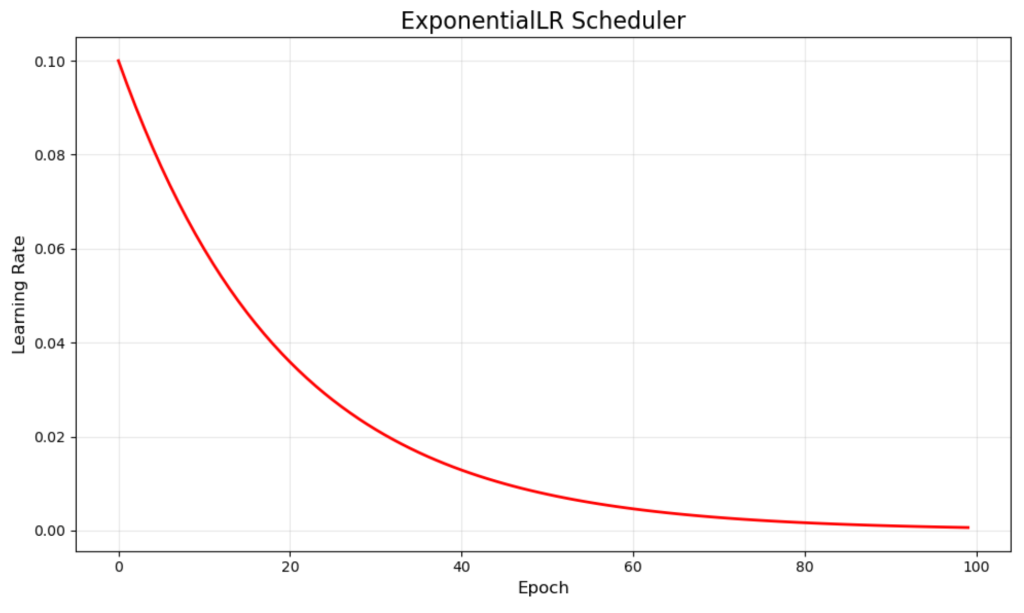
This continuous decay ensures the model consistently makes smaller and smaller updates as training progresses. It’s particularly effective for problems where you want gradual refinement without sharp transitions that might disrupt training momentum.

The smooth nature of exponential decay often leads to stable convergence, but requires careful tuning of the decay rate to avoid reducing the learning rate too quickly or too slowly.

CosineAnnealingLR – Cosine Annealing

CosineAnnealingLR follows a cosine curve, starting high and smoothly decreasing to a minimum value. The green curve shows this elegant mathematical progression, which naturally slows the rate of change as it approaches the minimum.

This scheduler is inspired by simulated annealing and has gained popularity in modern deep learning. The cosine shape provides more training time at higher learning rates early on, then gradually transitions to fine-tuning phases.

Research suggests cosine annealing can help models escape local minima and often achieves better final performance than linear decay schedules, especially in complex optimization landscapes.

ReduceLROnPlateau – Adaptive Plateau Reduction

ReduceLROnPlateau takes a different approach by monitoring validation metrics and reducing the learning rate only when improvement stagnates. The purple visualization shows typical behavior with reductions occurring around epochs 25, 50, and 75.

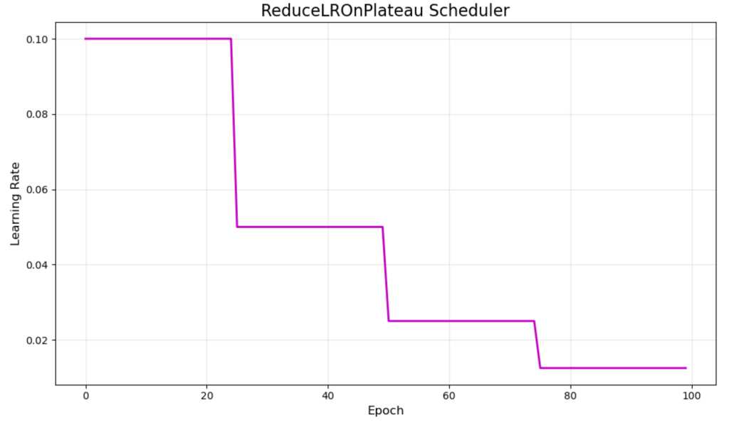
This adaptive scheduler responds to actual training progress rather than following a predetermined schedule. It reduces the learning rate when validation loss stops improving for a specified number of epochs (patience parameter).

The main strength is its responsiveness to training dynamics, making it excellent for cases where you’re unsure about optimal scheduling. However, it requires monitoring validation metrics and may react slowly to needed adjustments.

CyclicalLR – Cyclical Learning Rates

CyclicalLR oscillates between minimum and maximum learning rates in a triangular pattern. Our orange visualization shows these cycles, with the rate climbing from 0.001 to 0.1 and back down over 40-epoch periods.

This approach, pioneered by Leslie Smith, challenges the conventional wisdom of only decreasing learning rates. The theory suggests that periodic increases help the model escape poor local minima and explore the loss surface more effectively.

While cyclical learning rates can achieve impressive results and often train faster than traditional methods, they require careful tuning of the minimum, maximum, and cycle length parameters to work effectively.

Practical Implementation: MNIST Example

Now let’s see how these schedulers perform. We’ll train a simple neural network on the MNIST digit classification dataset to compare how different schedulers affect training performance.

Setup and Data Preparation

We start by importing the necessary libraries and preparing our data. The MNIST dataset contains handwritten digits (0-9) that we’ll classify using a basic two-layer neural network.

Our model is intentionally simple – a single hidden layer with 128 neurons. We use only 10,000 training samples to speed up the experiment while still demonstrating the schedulers’ behaviors.

Scheduler Implementations

Next, we implement each scheduler. Most schedulers can be implemented as simple functions that take the current epoch and learning rate, then return the new learning rate. However, ReduceLROnPlateau works differently since it needs to monitor validation metrics, so we’ll handle it separately in the training section.

Notice how each function implements the exact same behavior shown in our earlier visualizations. The parameters are carefully chosen to match those patterns. ReduceLROnPlateau requires special handling since it monitors validation loss during training, which you’ll see in the next section where we set it up as a callback.

Training and Comparison

We then create a training function that can use any of these schedulers and run experiments with each one: