
Mastering Time Series Forecasting: From ARIMA to LSTM
Image by Editor | Midjourney
Introduction
Time series forecasting is a statistical technique used to analyze historical data points and predict future values based on temporal patterns. This method is particularly valuable in domains where understanding trends, seasonality, and cyclical patterns drives critical business decisions and strategic planning. From predicting stock market fluctuations to forecasting energy demand spikes, accurate time series analysis helps organizations optimize inventory, allocate resources efficiently, and mitigate operational risks. Modern approaches combine traditional statistical methods with machine learning to handle both linear relationships and complex nonlinear patterns in temporal data.
In this article, we will explore three main methods for forecasting:
- Autoregressive Integrated Moving Average (ARIMA): A simple and popular method that uses past values to make predictions
- Exponential Smoothing Time Series (ETS): This method looks at trends and patterns over time to give better forecasts
- Long Short-Term Memory (LSTM): A more advanced method that uses deep learning to understand complex data patterns
Preparation
First, we import the required libraries.
|
# Import necessary libraries import pandas as pd import numpy as np import matplotlib.pyplot as plt from statsmodels.tsa.arima.model import ARIMA from statsmodels.tsa.stattools import adfuller from statsmodels.tsa.holtwinters import ExponentialSmoothing from prophet import Prophet from sklearn.model_selection import train_test_split from sklearn.preprocessing import MinMaxScaler from keras.models import Sequential from keras.layers import LSTM, Dense, Input |
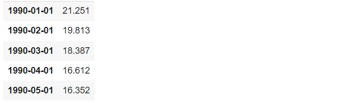
Then, we load the time series and view its first few rows.
|
# Load your dataset df = pd.read_csv(‘timeseries.csv’, parse_dates=[‘Date’], index_col=‘Date’) df.head() |
1. Autoregressive Integrated Moving Average (ARIMA)
ARIMA is a well-known method used to predict future values in a time series. It combines three components:
- AutoRegressive (AR): The relationship between an observation and a number of lagged observations
- Integrated (I): The differencing of raw observations to allow for the time series to become stationary
- Moving Average (MA): The relationship shows how an observation differs from the predicted value in a moving average model using past data
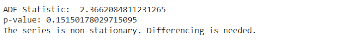
We use the Augmented Dickey-Fuller (ADF) test to check if our data stays the same over time. We look at the p-value from this test. If the p-value is 0.05 or lower, it means our data is stable.
|
# ADF Test to check for stationarity result = adfuller(df[‘Price’])
print(‘ADF Statistic:’, result[0]) print(‘p-value:’, result[1])
if result[1] > 0.05: print(“The series is non-stationary. Differencing is needed.”) else: print(“The series is stationary.”) |
We perform first-order differencing on the time series data to make it stationary.
|
# First-order differencing df[‘Differenced’] = df[‘Price’].diff()
# Drop missing values resulting from differencing df.dropna(inplace=True)
# Display the first few rows of the differenced data print(df[[‘Price’, ‘Differenced’]].head()) |

We create and fit the ARIMA model to our data. After fitting the model, we forecast the future values.
|
# Fit the ARIMA model model = ARIMA(df[‘Price’], order=(1, 1, 1)) model_fit = model.fit()
# Forecasting next steps forecast = model_fit.forecast(steps=10) |
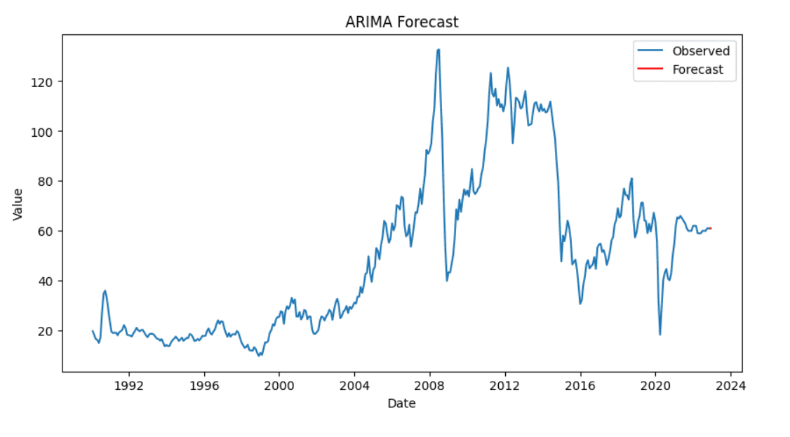
Finally, we visualize our results to compare the actual and predicted values.
|
# Plotting the results plt.figure(figsize=(10, 5)) plt.plot(df[‘Price’], label=‘Observed’) plt.plot(pd.date_range(df.index[–1], periods=10, freq=‘D’), forecast, label=‘Forecast’, color=‘red’) plt.title(‘ARIMA Forecast’) plt.xlabel(‘Date’) plt.ylabel(‘Value’) plt.legend() plt.show() |
2. Exponential Smoothing Time Series (ETS)
Exponential smoothing is a method used for time series forecasting. It includes three components:
- Error (E): Represents the unpredictability or noise in the data
- Trend (T): Shows the long-term direction of the data
- Seasonality (S): Captures repeating patterns or cycles in the data
We will use the Holt-Winters method for performing ETS. ETS helps us predict data that has both trends and seasons.
|
# Fit the ETS model (Exponential Smoothing) ets_model = ExponentialSmoothing(df[‘Price’], seasonal=‘add’, trend=‘add’, seasonal_periods=12) ets_fit = ets_model.fit() |
We generate forecasts for a specified number of periods using the fitted ETS model.
|
# Forecasting the next 12 periods forecast = ets_fit.forecast(steps=12) |
Then, we plot the observed data along with the forecasted values to visualize the model’s performance.
|
# Plot observed and forecasted values plt.figure(figsize=(10, 6)) plt.plot(df, label=‘Observed’) plt.plot(forecast, label=‘Forecast’, color=‘red’) plt.title(‘ETS Model Forecast’) plt.xlabel(‘Date’) plt.ylabel(‘Price’) plt.legend() plt.show() |

3. Long Short-Term Memory (LSTM)
LSTM is a type of neural network that looks at data in a sequence. It is good at remembering important details for a long time. This makes it useful for predicting future values in time series data because it can find complex patterns.
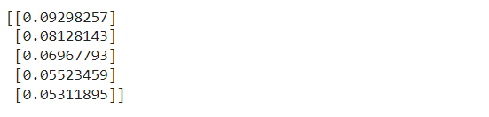
LSTM is sensitive to scale of the data. So, we adjust the target variable to make sure all values are between 0 and 1. This process is called normalization.
|
# Extract the values of the target column data = df[‘Price’].values data = data.reshape(–1, 1)
# Normalize the data scaler = MinMaxScaler(feature_range=(0, 1)) scaled_data = scaler.fit_transform(data)
# Display the first few scaled values print(scaled_data[:5]) |
LSTM expects input in the form of sequences. Here, we’ll split the time series data into sequences (X) and their corresponding next value (y).
|
# Create a function to convert data into sequences for LSTM def create_sequences(data, time_steps=60): X, y = [], [] for i in range(len(data) – time_steps): X.append(data[i:i+time_steps, 0]) y.append(data[i+time_steps, 0]) return np.array(X), np.array(y)
# Use 60 time steps to predict the next value time_steps = 60 X, y = create_sequences(scaled_data, time_steps)
# Reshape X for LSTM input X = X.reshape(X.shape[0], X.shape[1], 1) |
We split the data into training and test sets.
|
# Split the data into training and test sets (80% train, 20% test) train_size = int(len(X) * 0.8) X_train, X_test = X[:train_size], X[train_size:] y_train, y_test = y[:train_size], y[train_size:] |
We will now build the LSTM model using Keras. Then, we will compile it using the Adam optimizer and mean squared error loss.
|
1 2 3 4 5 6 7 8 9 10 11 12 13 14 15 16 17 |
from keras.models import Sequential from keras.layers import LSTM, Dense, Input
# Initialize the Sequential model model = Sequential()
# Define the input layer model.add(Input(shape=(time_steps, 1)))
# Add the LSTM layer model.add(LSTM(50, return_sequences=False))
# Add a Dense layer for output model.add(Dense(1))
# Compile the model model.compile(optimizer=‘adam’, loss=‘mean_squared_error’) |
We train the model using the training data. We also evaluate the model’s performance on the test data.
|
# Train the model on the training data history = model.fit(X_train, y_train, epochs=20, batch_size=32, validation_data=(X_test, y_test)) |
After we train the model, we will use it to predict the results on the test data.
|
# Make predictions on the test data y_pred = model.predict(X_test)
# Inverse transform the predictions and actual values to original scale y_pred_rescaled = scaler.inverse_transform(y_pred) y_test_rescaled = scaler.inverse_transform(y_test.reshape(–1, 1))
# Display the first few predicted and actual values print(y_pred_rescaled[:5]) print(y_test_rescaled[:5]) |

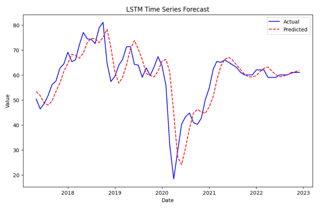
Finally, we can visualize the predicted values against the actual values. The actual values are shown in blue, while the predicted values are in red with a dashed line.
|
# Plot the actual vs predicted values plt.figure(figsize=(10,6)) plt.plot(df.index[–len(y_test_rescaled):], y_test_rescaled, label=‘Actual’, color=‘blue’) plt.plot(df.index[–len(y_test_rescaled):], y_pred_rescaled, label=‘Predicted’, color=‘red’, linestyle=‘dashed’) plt.title(‘LSTM Time Series Forecast’) plt.xlabel(‘Date’) plt.ylabel(‘Value’) plt.legend() plt.show() |
Wrapping Up
In this article, we explored time series forecasting using different methods.
We started with the ARIMA model. First, we checked if the data was stationary, and then we fitted the model.
Next, we used Exponential Smoothing to find trends and seasonality in the data. This helps us see patterns and make better forecasts.
Finally, we built a Long Short-Term Memory model. This model can learn complicated patterns in the data. We scaled the data, created sequences, and trained the LSTM to make predictions.
Hopefully this guide has been of use to you in covering these time series forecasting methods.