The Complete Guide to Feature Engineering for Better Model Performance
Feature engineering helps make models work better. It involves selecting and modifying data to improve predictions. This article explains feature engineering and how to use it to get better results.
What is Feature Engineering?
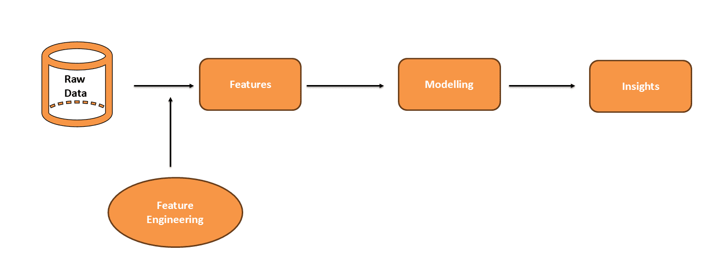
Raw data is often messy and not ready for predictions. Features are important details in your data. They help the model understand and make predictions. Feature engineering improves these features to make them more useful. Modeling uses these improved features to predict outcomes. Analyzing the model’s results provides insights. Well-engineered features make these insights clearer. This helps you understand data patterns better and improves model performance.


Why is Feature Engineering Important?
- Improved Accuracy: Good features help the model learn better patterns. This leads to more accurate predictions.
- Reduced Overfitting: Better features help the model generalize well to new data. This reduces the chance of overfitting.
- Algorithm Flexibility: Many algorithms work better with clean and well-prepared features.
- Easy Interpretability: Clear features make it easier to understand how the model makes decisions.
Feature Engineering Processes
Feature engineering can involve several processes:
- Feature Extraction: Make new features from what you already have. Use methods like PCA or embeddings to do this.
- Feature Selection: Choose the most important features to help your model work better. This keeps the model focused on the important details.
- Feature Creation: Create new features from existing ones to help the model make better predictions. This gives the model more useful information.
- Feature Transformation: Modify features to make them more suitable for the model. Normalization scales values to be within a range of 0 to 1. Standardization adjusts features to have a mean of 0 and a standard deviation of 1.
Feature Engineering Techniques
Let’s discuss some of the common techniques of feature engineering.
Handling Missing Values
It’s important to handle missing data is for making accurate models. Here are some ways to remove them:
- Imputation: Use methods like mean, median, or mode to fill in missing values based on other data in the column.
- Deletion: Remove rows or columns with missing values if the amount is small and won’t significantly impact the analysis.
|
1 2 3 4 5 6 7 8 9 10 11 12 13 14 15 16 17 18 19 20 |
import pandas as pd from sklearn.impute import SimpleImputer
# Load data from a CSV file df = pd.read_csv(‘data.csv’)
# Print data before imputation print(“Data before cleaning:”) print(df.head())
# Remove commas from ‘Salary’ column and convert to numeric df[‘Salary’] = df[‘Salary’].str.replace(‘,’, ”).astype(float)
# Impute missing numerical values with the median imputer = SimpleImputer(strategy=‘median’) df[[‘Age’, ‘Salary’]] = imputer.fit_transform(df[[‘Age’, ‘Salary’]])
# Print data after imputation print(“\nData after imputing missing values:”) print(df.head()) |
The missing values in the “Age” and “Salary” columns are filled in with the median values.


Encoding Categorical Variables
Categorical variables need to be converted into numerical values for machine learning models. Here are some common methods:
- One-Hot Encoding: Generate new columns for each category. Each category gets its own column with a 1 or 0.
- Label Encoding: Give each category a distinct number. Useful for ordinal data where the order matters.
- Binary Encoding: Convert categories to binary numbers and then split into separate columns. This method is useful for high-cardinality data.
|
import pandas as pd from sklearn.preprocessing import LabelEncoder
# Load the dataset df = pd.read_csv(‘data.csv’)
# One-Hot Encoding for the Department column df = pd.get_dummies(df, columns=[‘Department’], drop_first=True)
# Display the data after encoding print(“Data after encoding categorical variables:”) print(df.head()) |
After one-hot encoding, the “Department” column is divided into new columns. Each column represents a category with binary values.


Binning
Binning groups continuous values into discrete bins or ranges. It simplifies the data and can help with noisy data.
- Equal-Width Binning: Divide the range into equal-width intervals. Each value falls into one of these intervals.
- Equal-Frequency Binning: Divide data into bins so each bin has roughly the same number of values.
|
import pandas as pd
# Load the dataset df = pd.read_csv(‘data.csv’)
# Binning Age into 3 categories (Young, Middle-Aged, Senior) df[‘Age_Binned’] = pd.cut(df[‘Age’], bins=3, labels=[‘Young’, ‘Middle-Aged’, ‘Senior’])
# Display the Age and Age_Binned columns (first 5 rows) print(“Data after binning Age (first 5 rows):”) print(df[[‘Age’, ‘Age_Binned’]].head()) |
Here, age is categorized into “Young,” “Middle-Aged,” or “Senior” based on the binning.


Handling Outliers
Outliers are data points that are different from the rest. They can mess up results and affect how well a model works. Here are some common ways to handle outliers:
- Removal: Exclude extreme values that don’t fit the overall pattern.
- Capping: Limit extreme values to a maximum or minimum threshold.
- Transformation: Use techniques like log transformation to reduce the impact of outliers.
|
1 2 3 4 5 6 7 8 9 10 11 12 13 14 15 16 17 18 19 20 21 22 23 24 25 26 27 |
import pandas as pd import numpy as np from scipy import stats
# Load the dataset df = pd.read_csv(‘data.csv’)
# Remove commas from ‘Salary’ column and convert to numeric df[‘Salary’] = df[‘Salary’].str.replace(‘,’, ”).astype(float)
# Detect Outliers using Interquartile Range (IQR) method Q1 = df[‘Salary’].quantile(0.25) Q3 = df[‘Salary’].quantile(0.75) IQR = Q3 – Q1
# Define outlier boundaries lower_bound = Q1 – 1.5 * IQR upper_bound = Q3 + 1.5 * IQR
# Identify outliers df[‘IQR_Outlier’] = (df[‘Salary’] < lower_bound) | (df[‘Salary’] > upper_bound)
# Remove outliers based on IQR df_cleaned_iqr = df[~df[‘IQR_Outlier’]]
# Print the first 5 rows of the cleaned data after removing outliers print(df_cleaned_iqr.head()) |
The output displays the dataset after removing outliers based on the Interquartile Range (IQR) method. These rows no longer include any entries with salaries outside the defined outlier boundaries.


Scaling
Scaling adjusts the range of feature values. It ensures that features contribute equally to model training.
- Normalization: Rescales values to a range, often 0 to 1. Example: Min-Max scaling.
- Standardization: Centers values around a mean of 0 and scales by the standard deviation. Example: Z-score normalization.
|
1 2 3 4 5 6 7 8 9 10 11 12 13 14 15 16 17 18 19 20 21 22 23 24 25 26 27 28 |
import pandas as pd from sklearn.preprocessing import MinMaxScaler, StandardScaler
# Load the dataset df = pd.read_csv(‘data.csv’)
# Remove commas from ‘Salary’ column and convert to numeric df[‘Salary’] = df[‘Salary’].str.replace(‘,’, ”).astype(float)
# Normalize features (Min-Max Scaling) min_max_scaler = MinMaxScaler() df[[‘Salary_Norm’, ‘Age_Norm’]] = min_max_scaler.fit_transform(df[[‘Salary’, ‘Age’]])
# Standardize features (Z-score Normalization) standard_scaler = StandardScaler() df[[‘Salary_Std’, ‘Age_Std’]] = standard_scaler.fit_transform(df[[‘Salary’, ‘Age’]]
# Print first 5 rows of original data print(“Original Data:”) print(df[[‘EmployeeID’, ‘Salary’, ‘Age’]].head())
# Print first 5 rows after normalization print(“\nData after normalization (Min-Max Scaling):”) print(df[[‘EmployeeID’, ‘Salary_Norm’, ‘Age_Norm’]].head())
# Print first 5 rows after standardization print(“\nData after standardization (Z-score Normalization):”) print(df[[‘EmployeeID’, ‘Salary_Std’, ‘Age_Std’]].head()) |
The code normalizes “Salary” and “Age” using Min-Max scaling, resulting in Salary_Norm and Age_Norm. It also standardizes these features using Z-score normalization.


Best Practices for Feature Engineering
Here are some tips to improve feature engineering:
- Iterate and Experiment: Feature engineering is often an iterative process. Test different transformations and interactions and validate them using cross-validation.
- Automate with Tools: Use tools like Featuretools for automated feature engineering or AutoML frameworks that perform feature selection and transformation.
- Understand the Feature’s Impact: Always track the impact of new features on model performance. Sometimes, a complex feature may not provide as much benefit as expected.
- Leverage Domain Knowledge: Incorporate insights from domain experts to create features that capture industry-specific patterns and nuances. This can provide valuable context and improve model relevance.
Conclusion
Feature engineering helps improve machine learning models. It makes your data more useful. By creating and selecting the right features, you get better predictions. This process is key for successful machine learning.
